Determinants and Eigenvectors
Eigenvalues and Eigenvectors
Dimensionality Reduction and Projection


Dimensionality reduction helps preserve information and helps with visualization in exploratory analysis.
Without it, we would be removing features that lead to losing information.
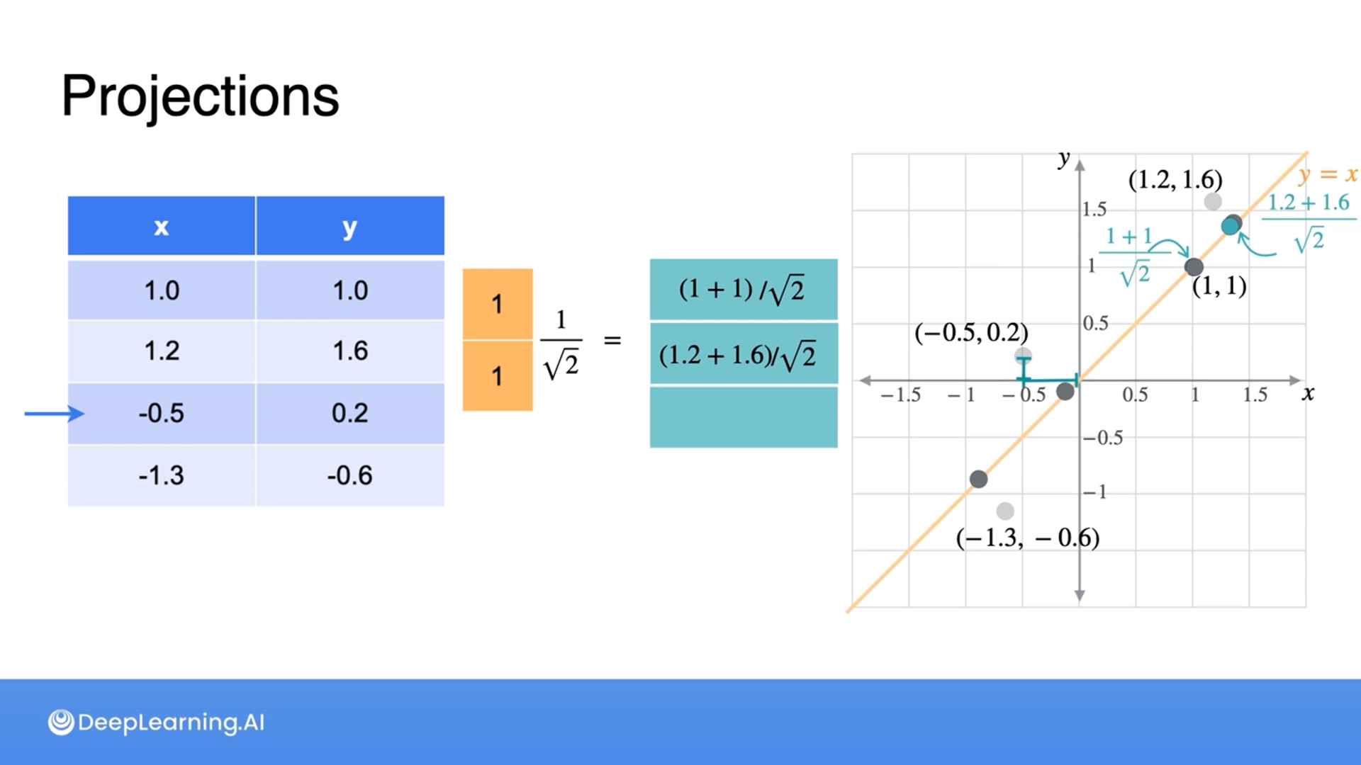
Projection: Moving data points into a vector space in different dimensions
Here we are talking about dimensionality reduction, hence fewer dimensions, but in practice, projection can be referred to as either fewer/lower or more/higher dimensions.
The main idea of the projection is that multiplying by the vector projects the points along that vector and dividing by the vector’s norm ensures that there’s no stretching introduced.
- Changing the vector to have a new norm of 1
For a quick recap, L2-norm is a square root of the sum of the squared data points.
$L_2 = \sqrt{x_1^2 + x_2^2 \dots x_n^2}$
Motivating PCA


We can project data points in any vectors.
To preserve the most information we need to find the line/vector that has the most spread between projected data points.
So less information if less spread and more information if more spread between projected data points.
Hence, the goal of PCA is to find the projection that preserves the maximum possible spread in the data while reducing the dimensionality.
Variance and Covariance
Few concepts of statistics are used for PCA


Mean: The average of the data
Variance: The spread between data
- Variance can be thought of as the average squared distance from the mean

The mean and variance themselves won’t explain the patterns of the data, hence covariance is used.
Covariance helps measure how two features of a dataset vary from one another.


The formula of the covariance shows we take the average of the sum of products of data minus the mean, so to simplify, which quadrants have more data and that shows the result of either positive covariance or negative covariance.
So we can think of covariance as the direction of the relationship between two variables.
Covariance Matrix


Covariance measures the relationship between pairs of variables in a dataset.
The covariance matrix stores the covariances and variances for each pair of variables.
The process of building a covariance matrix involves calculating the variances and covariances of the variables.
The covariance matrix can be expressed in matrix notation for efficient computation.
The matrix multiplication of the transpose of the matrix of observations and the matrix of mean values gives the covariance matrix.
Here’s an example of getting a covariance matrix:


Getting the covariance matrix of more than 2 variables is not any different from computing a covariance matrix of two variables.
PCA - Overview

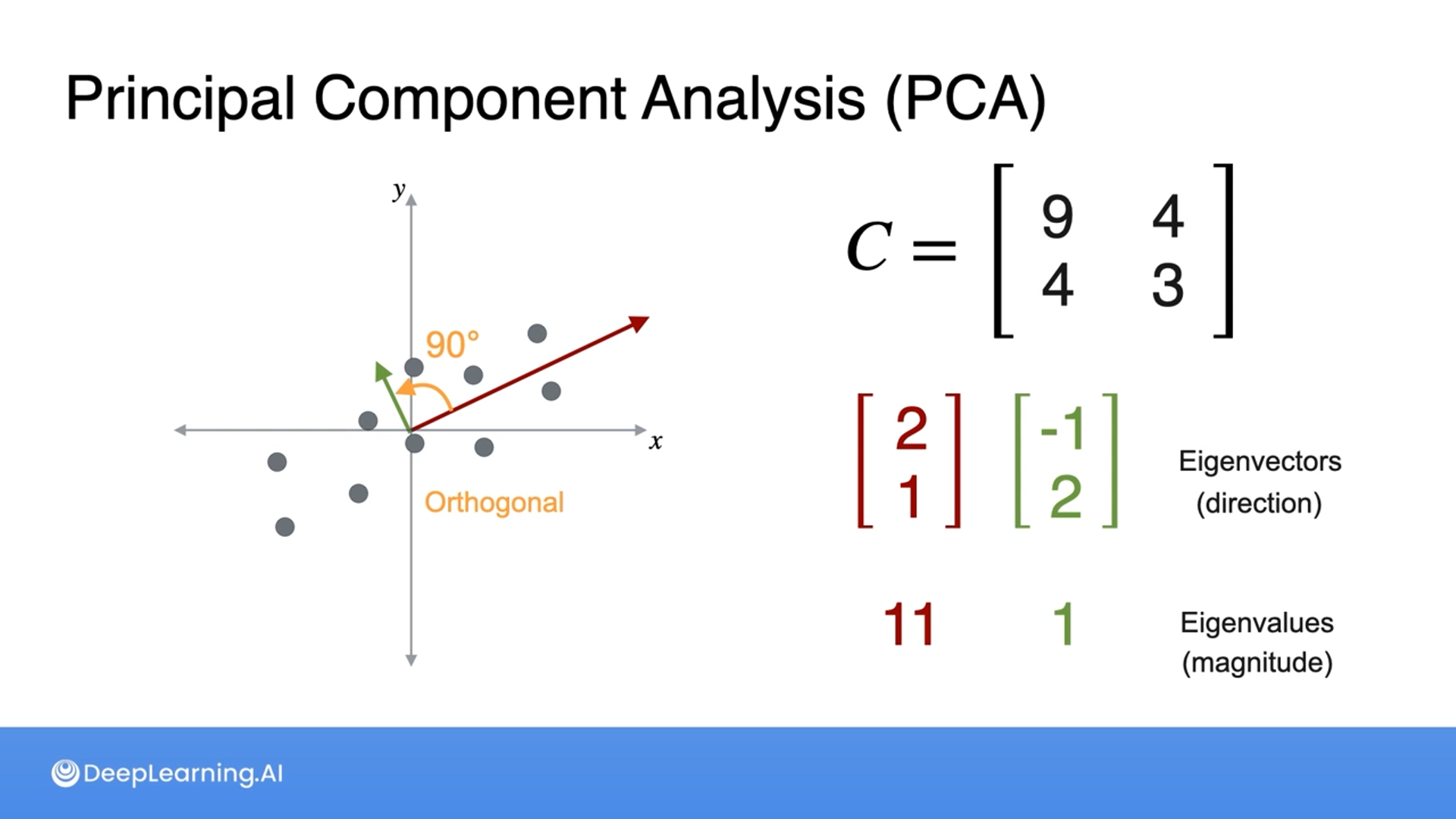


A way to find the best line/vector that captures the most variance (information) is by PCA, which combines concepts like projections, eigenvalues, eigenvectors, and covariance matrices.
Projection allows us to use a simple matrix multiplication to project data into a lower dimensional space.
Eigenvalues/eigenvectors capture the directions in which a linear transformation only stretches space but doesn’t rotate or shear it.
The covariance matrix compactly represents relationships between the variables in the dataset.
The steps for PCA are:
- Center the data so the mean of the data is at 0
- Find the covariance matrix
- Find the eigenvalues and eigenvectors of the covariance matrix
- The vectors we find are orthogonal (90 degrees to one another)
- The largest eigenvalue will have the most spread (variance) when the data is projected, so choose the eigenvector with the largest eigenvalue
- The data is then projected onto this line, reducing its dimensionality (this is done through the dot product of the original matrix by the eigenvectors
The goal of PCA is to reduce the dimensionality of data while preserving as much variance as possible.
PCA - Why It Works
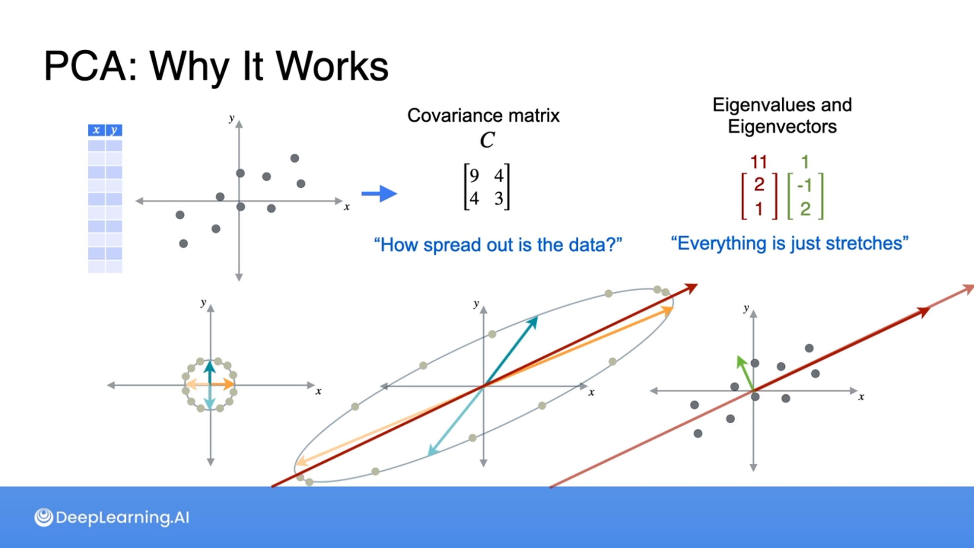

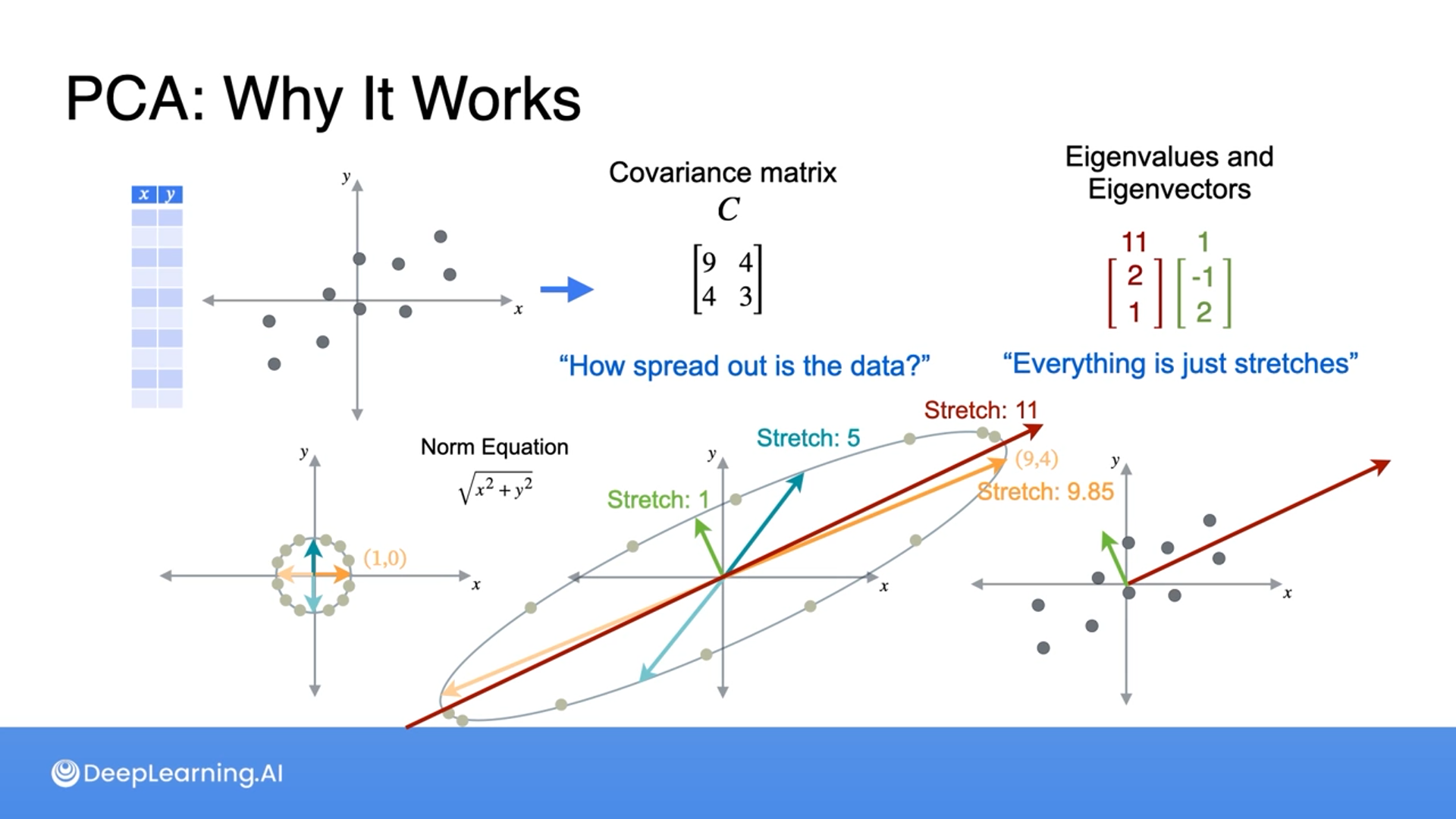
A covariance matrix is how spread out the data is so we can think of a covariance matrix as a change of basis.
Then we utilize eigenvalues and eigenvectors to choose the best line that preserves the most spread (information).
This can be explained with linear transformation as how much the points stretch by (stretch by a factor of what).
For instance, an orange vector (1, 0) gets stretched by 9.85, to (9, 4) and a teal vector (0, 1) gets stretched by 5, to (4, 3).
Any other eigenbases between would have fewer eigenvalues than the largest one, hence we choose the eigenvector with the largest eigenvalue.
PCA - Mathematical Formulation


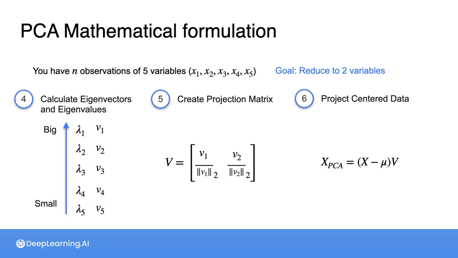
The steps to using PCA:
- Create a matrix
- Center your data (matrix) by subtracting the column average from each data
- Calculate covariance matrix
- Calculate eigenvectors and eigenvalues then sort by eigenvalues
- Create a projection matrix
- Choose how much to reduce the data’s dimensionality
- If reduced to 2 dimensions, we’ll choose 2 eigenvalues that are the largest and use their eigenvectors scaled by their norms
- $V= \left[\begin{array}{cc}{v_1 \over ||v_1||_2}&{v_2\over ||v_2||_2}\end{array}\right]$
- Choose how much to reduce the data’s dimensionality
- Project the centered data by multiplying centered data by projection matrix $V$
- $X_{PCA}=(X-\mu)V$
Discrete Dynamical Systems


It’s a fairly straightforward application of eigenvectors.
A Markov matrix is a square matrix with non-negative values that add up to one, representing the probabilities of transitioning between different states.
This is important because it allows us to infer the probability of how the system will evolve.
The state vector represents the current state of the system, and by taking the dot product with the Markov matrix, we can predict the probabilities of transitioning to different states in the future.
To get the data after, we use the output of the previous state vector as the new state vector and perform a dot product with the original data (matrix).
As we iterate this process, the state vectors tend to stabilize, and we reach an equilibrium vector that represents the long-run probabilities of each state.
The equilibrium vector is also an eigenvector of the transition matrix.
All the information here is based on the Linear Algebra for Machine Learning and Data Science | Coursera from DeepLearning.AI
'Coursera > Mathematics for ML and Data Science' 카테고리의 다른 글
| Calculus for Machine Learning and Data Science (0) (0) | 2024.08.21 |
|---|---|
| Linear Algebra for Machine Learning and Data Science (17) (0) | 2024.08.20 |
| Linear Algebra for Machine Learning and Data Science (15) (0) | 2024.06.07 |
| Linear Algebra for Machine Learning and Data Science (14) (0) | 2024.06.05 |
| Linear Algebra for Machine Learning and Data Science (13) (0) | 2024.06.04 |


