Neural Networks Basics
Set up a machine learning problem with a neural network mindset and use vectorization to speed up your models.
Learning Objectives
- Build a logistic regression model structured as a shallow neural network
- Build the general architecture of a learning algorithm, including parameter initialization, cost function, gradient calculation, and optimization implementation (gradient descent)
- Implement computationally efficient and highly vectorized versions of models
- Compute derivatives for logistic regression, using a backpropagation mindset
- Use Numpy functions and Numpy matrix/vector operations
- Work with iPython Notebooks
- Implement vectorization across multiple training examples
- Explain the concept of broadcasting
Logistic Regression as a Neural Network
Binary Classification

Our goal with binary classification is to classify data into two classes, usually 0 or 1.
Logistic Regression

Given X, we want to find $\hat y$ or the probability of target (y) = 1 and we can get this by using a formula from linear algebra: y = ax + b (in AI, we use y = wx + b).
We use parameters w (weights) and b (bias) to multiply our data to get the prediction.
We apply a sigmoid function to our formula (in the slide) to ensure our predicted output falls within 0 and 1.
What are the parameters of logistic regression?
W, an $n_x$ dimensional vector, and b, a real number.
Logistic Regression Cost Function

We’d think that square loss is a reasonable way to approach a loss function, but it doesn’t work well on gradient descent during optimization due to being non-convex with possibly multiple local optima.
What is the difference between the cost function and the loss function for logistic regression?
The loss function computes the error for a single training example; the cost function is the average of the loss functions of the entire training set.
Gradient Descent


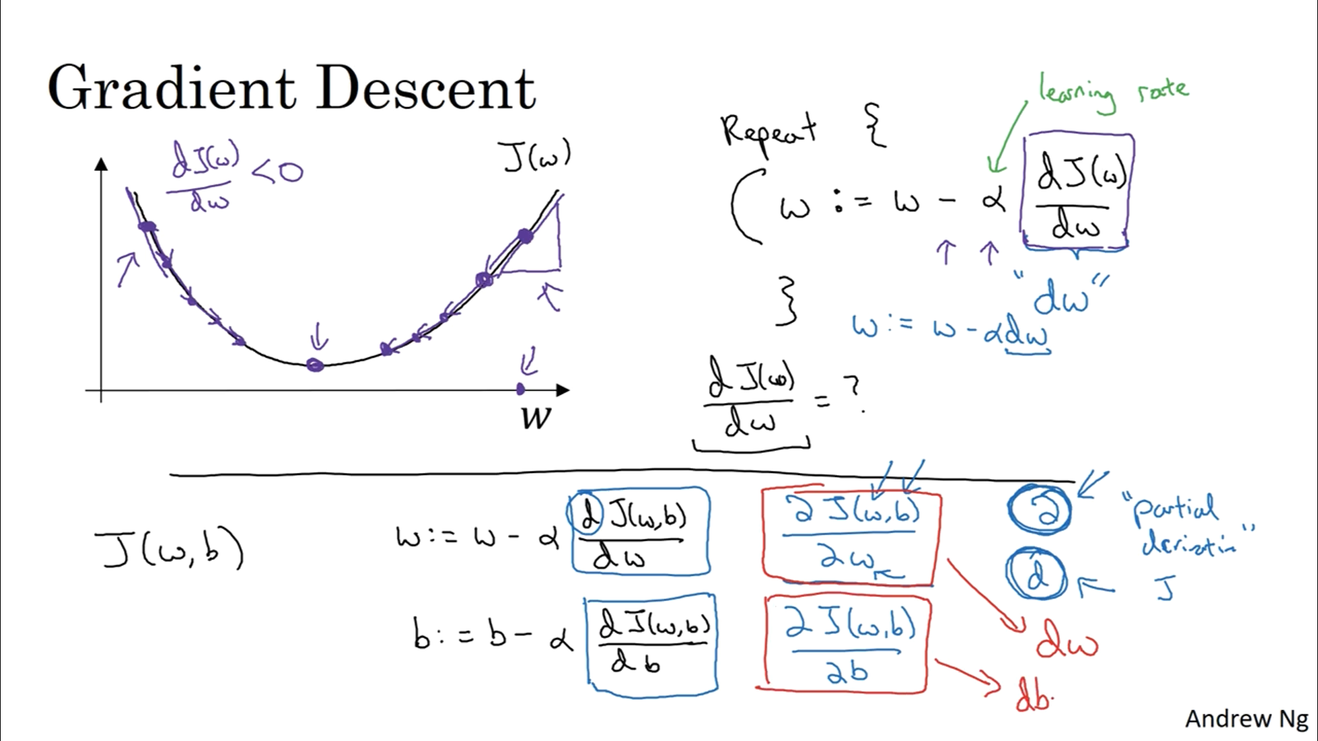
We initialize our parameters w and b with some values and try to find the minimum value for the loss function.
For logistic regression, we can initialize our w and b because the loss function has a convex shape.
For other loss functions, we initialize w and b with random values.
We use gradient descent to iterate the process of updating parameters to find the global optimum.
To update, we take partial derivatives of the parameters multiplied by the learning rate.
The learning rate is set to update our parameters not too slowly or drastically toward where the gradient is heading.
True or false. A convex function always has multiple local optima.
False
Derivatives

Derivative can also be thought of as a slope (height over width).
It tells us how much height moves if we change/update our width.
So the function of variable (a) is the height and a variable (a) is the width.
On a straight line, the function's derivative…
doesn’t change
More Derivative Examples


If the function is not a straight line, depending on the location, the value of the function changes instead of increasing at a constant level.
With our example $a^2$, the derivative is 2a, so depending on the value, the function outputs a different value instead of constantly increasing by 4 times.
So the derivative tells us how much the function (height) moves when the value (width) moves by some amount.
And we can think of the derivative as a slope of the line (how much we moved a point).
All the information provided is based on the Deep Learning Specialization | Coursera from DeepLearning.AI
'Coursera > Deep Learning Specialization' 카테고리의 다른 글
| Neural Networks and Deep Learning (4) (0) | 2024.11.17 |
|---|---|
| Neural Networks and Deep Learning (3) (0) | 2024.11.14 |
| Neural Networks and Deep Learning (1) (1) | 2024.11.12 |
| Neural Networks and Deep Learning (0) (4) | 2024.11.11 |
| Deep Learning Specialization (1) | 2024.11.10 |


