▤ 목차
Practical Aspects of Deep Learning
Regularizing your Neural Network
Clarification about Upcoming Regularization Video
Please note that in the next video (Regularization) at 5:45, the Frobenius norm formula should be the following:
$∣∣w^{[l]}∣∣^2=∑_{i=1}^{n^{[l]}}∑_{j=1}^{n^{[l−1]}}(w_{i,j}^{[l]})^2$
The limit of summation of i should be from 1 to $n^{[l]}$,
The limit of summation of j should be from 1 to $n^{[l-1]}$.
(It’s flipped in the video).
The rows "i" of the matrix should be the number of neurons in the current layer $n^{[l]}$;
whereas the columns "j" of the weight matrix should equal the number of neurons in the previous layer $n^{[l-1]}$.
Regularization


Regularization is one way to prevent overfitting without getting more data.
$\lambda$ is the regularization parameter (hyperparameter).
Logistic regression
L2 regularization is the most common type of regularization
- Use norm 2
- The Euclidean norm which is the weight matrix transposed multiplied by the weight matrix
- We usually omit to regularize the parameter $b$
- $b$ is just a single parameter whereas the parameter $w$ is a high-dimensional vector, which means if you regularize $b$, we are regularizing a single number (1 parameter), so it wouldn’t help much
- But if you want, you can
L1 regularization
- $w$ will be sparse (lots of zeros), some say it will help compress the model
- It doesn’t help in terms of regularization
Neural network
Use “Frobenius norm” for the regularization
- The squared norm (all of the elements squared)
- By convention (for arcane reasons) it’s called the Frobenius norm instead of the L2 norm
- A sum of squares of the matrix
- To perform a gradient descent, during the backpropagation of the weights, we add the regularization
- aka “weight decay” because we are multiplying the weight matrix by a number slightly less than 1
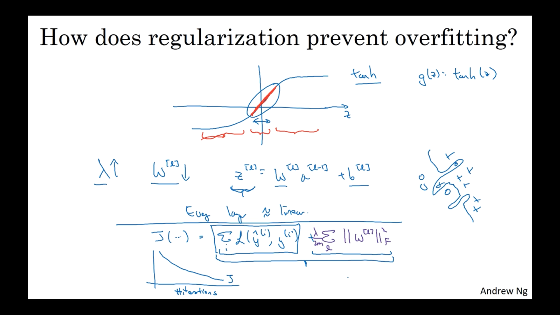
Why Regularization Reduces Overfitting?


Regularization penalizes the weight matrices from being too large.
If $\lambda$ is big, the weights will get close to zero, so we are simplifying the neural network (zeroing out the impact of several hidden units).
Another example is given by using a tanh function
- If z is small, then the tanh of z becomes roughly linear as if it’s a linear regression
Strengthening $\lambda$ via regularization updates weights smaller than the ones without regularization, so the impact of the weights is less and leads to a reduction in the variance.
Dropout Regularization


A technique to kill nodes of each layer based on probability to prevent overfitting and killing different nodes for each training example (not killing the same nodes only).
# Illustrated with layer l = 3 and keep_prob = 0.8
l = 3
keep_prob = 0.8 # means 80% keeping node and 20% killing node
d3 = np.random.rand(a3.shape[0], a3.shape[1]) < keep_prob
a3 = np.multiply(a3, d3) # a3 *= d3

# inverted dropout
# ensures the expected value of a3 remains the same for the next layer
a3 /= keep_prob
Making predictions at test time
Using dropout at test time adds noise to the predictions, so avoid using dropout at test time.
Clarification about Upcoming Understanding Dropout Video
Please note that in the next video from around 2:40 - 2:50, the dimension of $w^{[1]}$ should be 7x3 instead of 3x7, and $w^{[3]}$ should be 3x7 instead of 7x3.
In general, the number of neurons in the previous layer gives us the number of columns of the weight matrix, and the number of neurons in the current layer provides us with the number of rows in the weight matrix.
Understanding Dropout

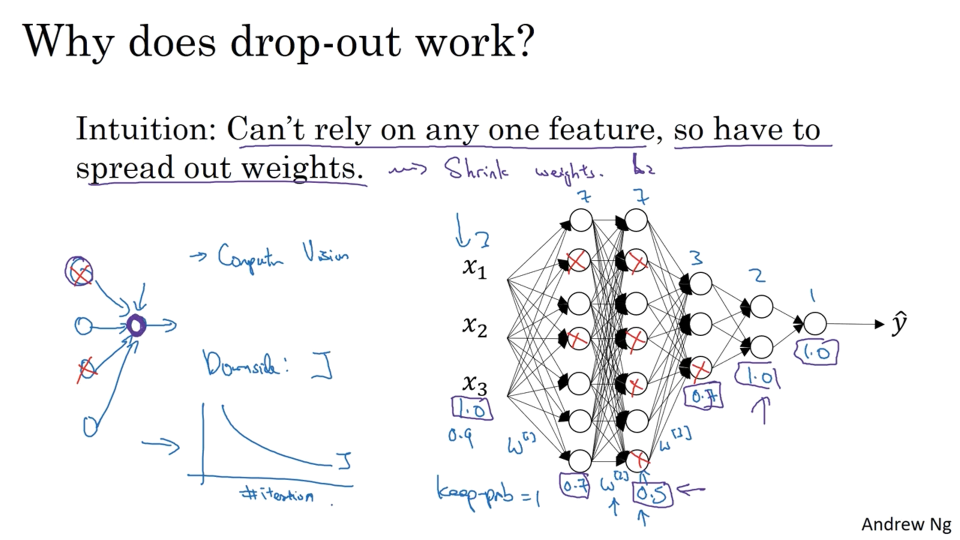
Why does drop-out work?
Intuition: Can’t rely on any one feature, so have to spread out weights
The nodes can be shut off at any time the impact of the weights spread out.
Can apply a lower threshold (set the lower probability) on the layers with more nodes than the layers with smaller nodes.
Commonly used on computer vision as input features are pixels of image and you seldom run short on features.
One downside of dropout is that your cost function $J$ is no longer well-defined
- Randomly killing random nodes makes it harder to check gradient descent
- So run the code without dropout (set keep_prob = 1) and check $J$ by plotting it, then apply dropout to reduce the variance
Other Regularization Methods


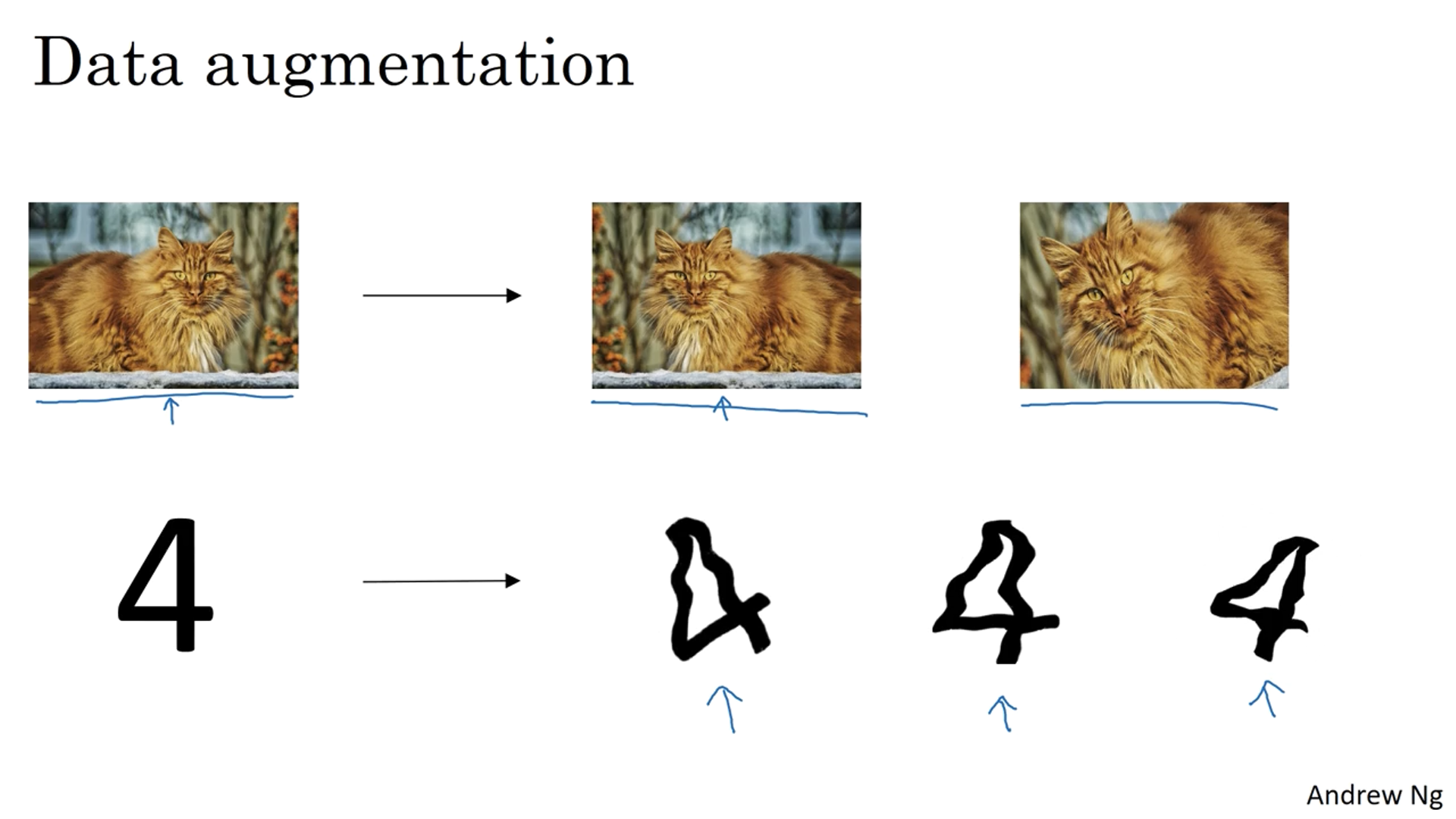
Data augmentation
For instance flipping, randomly cropping an image, and putting it to the training set prevents overfitting. It is also better than finding data outside.
For optical data, slight distortion can help, like cursive or squiggles of numbers.
Early stopping
Plot training set and dev set errors.
Stop training your network when the dev set error increases instead of decreasing.
The downside of early stopping is that one is using one tool to solve two different problems (optimize cost function $J$ and not overfit)
- Not able to optimize cost function as much compared to not using early stopping
Advantage of early stopping
- Quicker to train
- Try different weights
Andrew Ng prefers using L2 regularization
- The downside of regularization is that the search space gets bigger (another hyperparameter to find on top of others)
All the information provided is based on the Deep Learning Specialization | Coursera from DeepLearning.AI
'Coursera > Deep Learning Specialization' 카테고리의 다른 글
| Improving Deep Neural Networks: Hyperparameter Tuning, Regularization, and Optimization (0) (1) | 2024.12.05 |
|---|---|
| Neural Networks and Deep Learning (11) (1) | 2024.12.04 |
| Neural Networks and Deep Learning (10) (0) | 2024.11.28 |
| Neural Networks and Deep Learning (9) (1) | 2024.11.27 |
| Neural Networks and Deep Learning (8) (1) | 2024.11.26 |


 }
}