Sampling and Point estimation
Point Estimation
Point Estimation
The most common point estimation method is maximum likelihood estimation (MLE), which is very popular in machine learning.
MLE can be generalized using Bayes’ theorem to a Bayesian version of a point estimator called the maximum a posteriori estimation.
MAP or maximum a posteriori estimation can be thought of as a maximum likelihood estimate with regularization.
Regularization is a commonly used method in machine learning to prevent overfitting.
Maximum Likelihood Estimation: Motivation
MLE is widely used in machine learning and the concept is simple, maximizing a conditional probability
Imagine you walk into your living room and see a bunch of popcorn lying on the floor next to the couch. Which one do you think is more likely to have happened?
- People were playing board games.
- People were taking a nap.
- People were watching a movie.
3
That's correct! You're more likely to eat popcorn watching a movie than playing board games or taking a nap.


With linear regression, we are trying to find a model that fits a straight line as close as possible to the data.
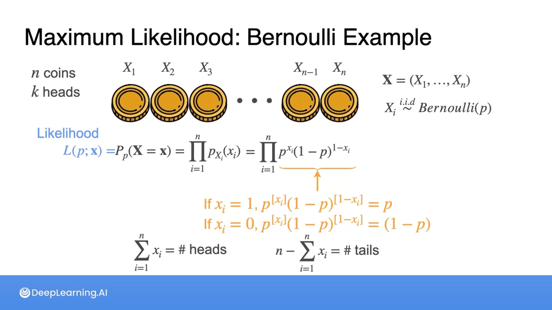
MLE: Bernoulli Example

Which coin is more likely to have generated the sequence of heads and tails above?
Coin 1
That's correct! You saw a lot of heads in the 10 tosses, and coin 1 is the one with the highest probability of seeing heads.

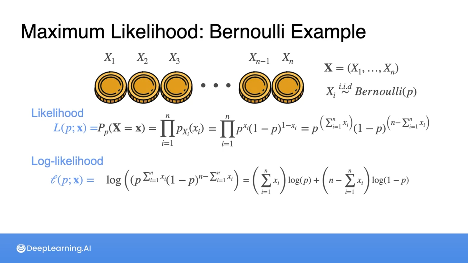
What operation can be done to the function $p^8(1-p)^2$ to find the maximum likelihood?
- Take the square root of the function.
- Take the natural logarithm of the function.
- Divide the function by 2.
2
Great job! Taking the natural logarithm of the function simplifies the expression by transforming products into sums, which makes differentiation easier. This aids in finding the maximum likelihood estimate for p.

Often we’ll see more log-likelihood than the maximum likelihood.
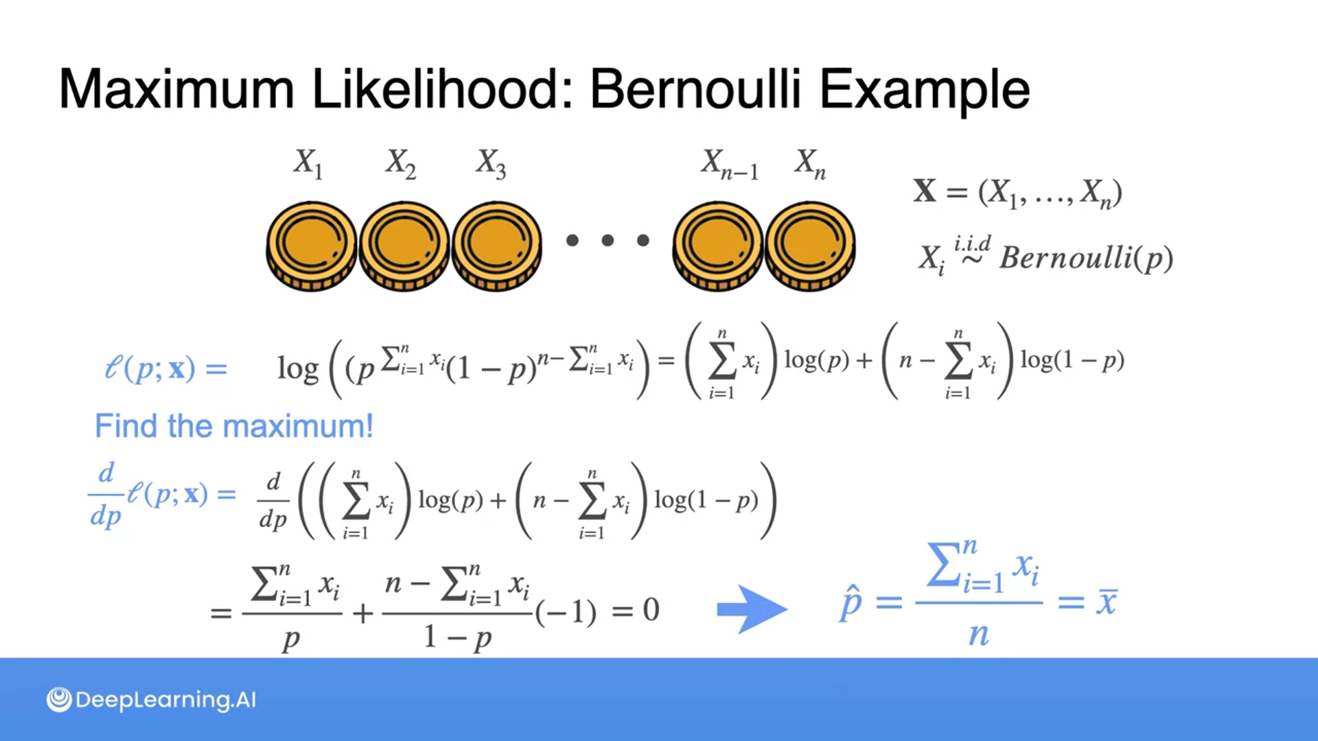
The optimal maximum value for the probability comes out to be the population mean.
So if we have k heads among the population of coins, then the optimal probability to obtain those k heads would be precisely k over n.
MLE: Gaussian Example
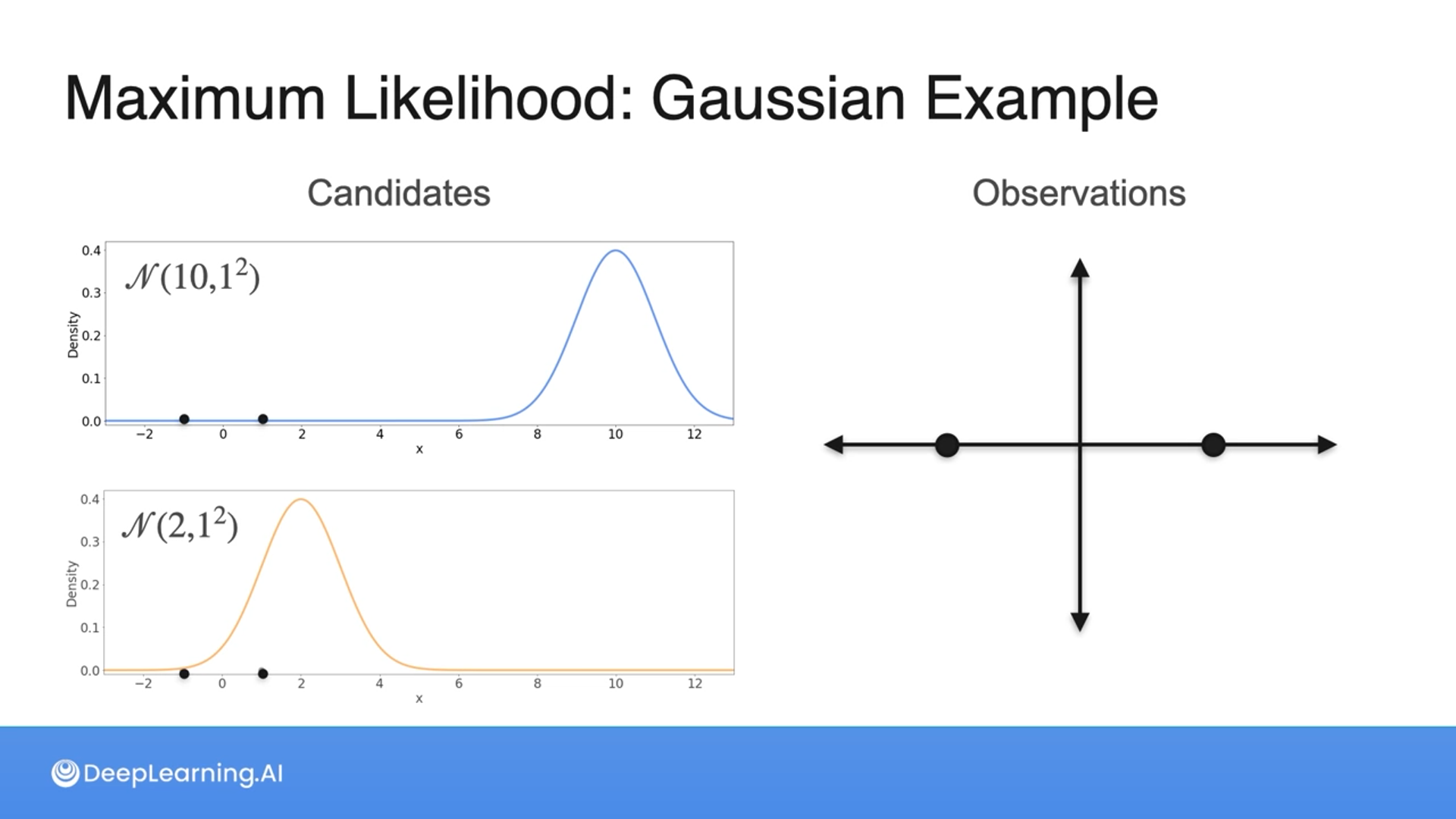
Given the sample {-1, 1} from an unknown Normal distribution, which one is more likely to have generated the sample?
- $N(10,1^2)$
- $N(2,1^2)$
2
Correct! Of the two possibilities given, the Gaussian with mean 2 and variance 1 maximizes the chances of seeing the sample {-1, 1}
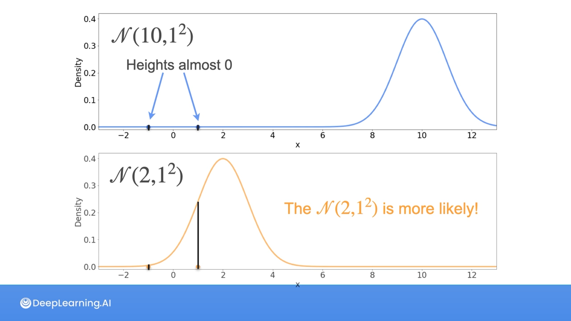
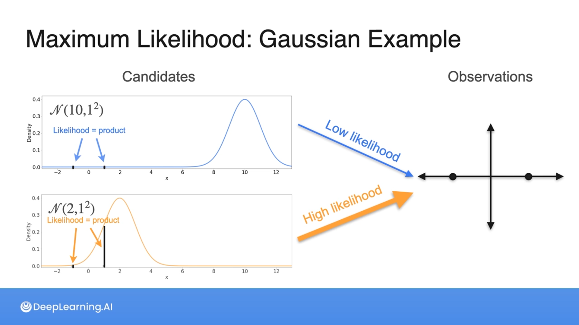
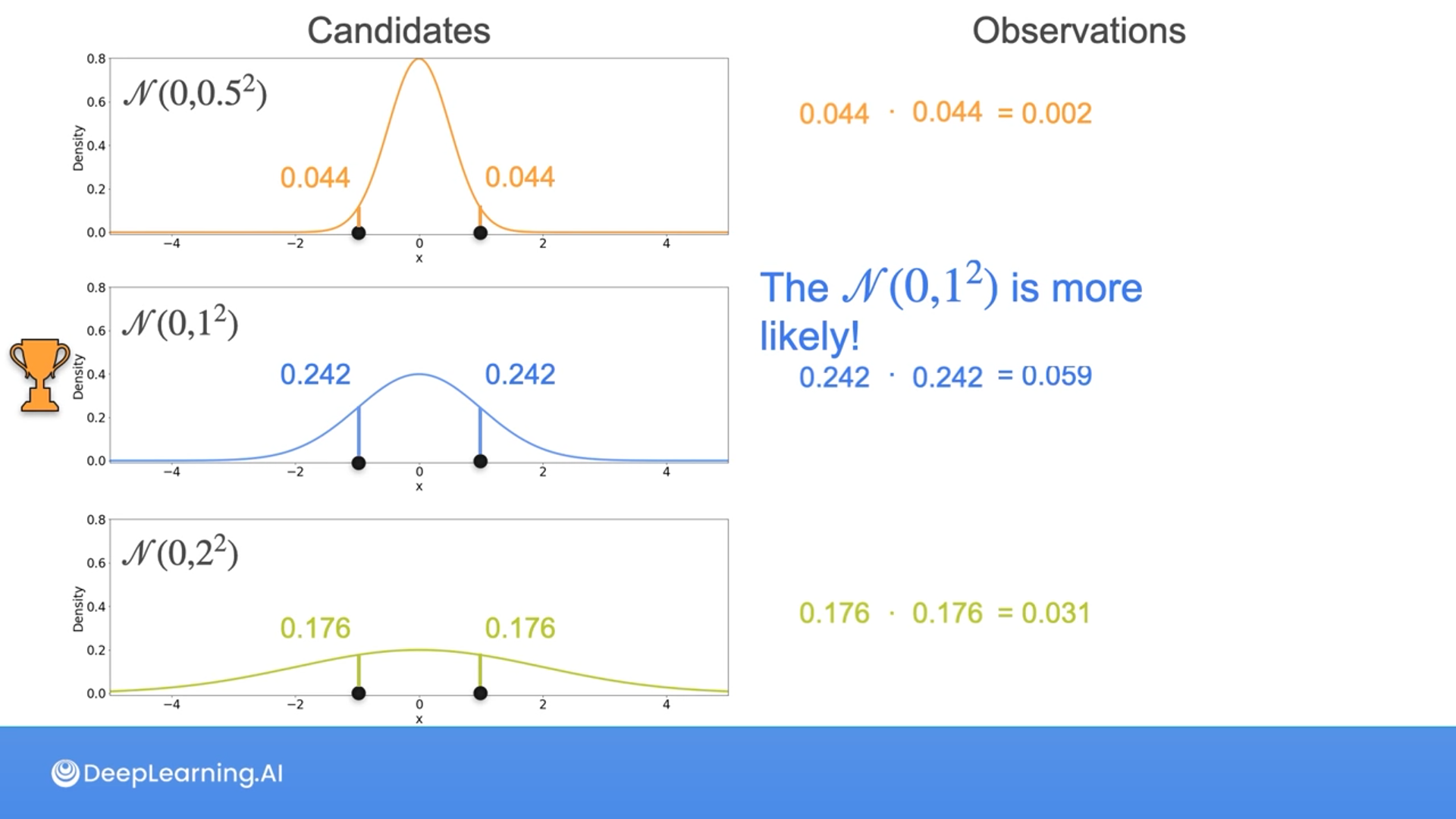
The heights are indicated as the likelihood and we take the product of the likelihood to find which one is higher or more likely.
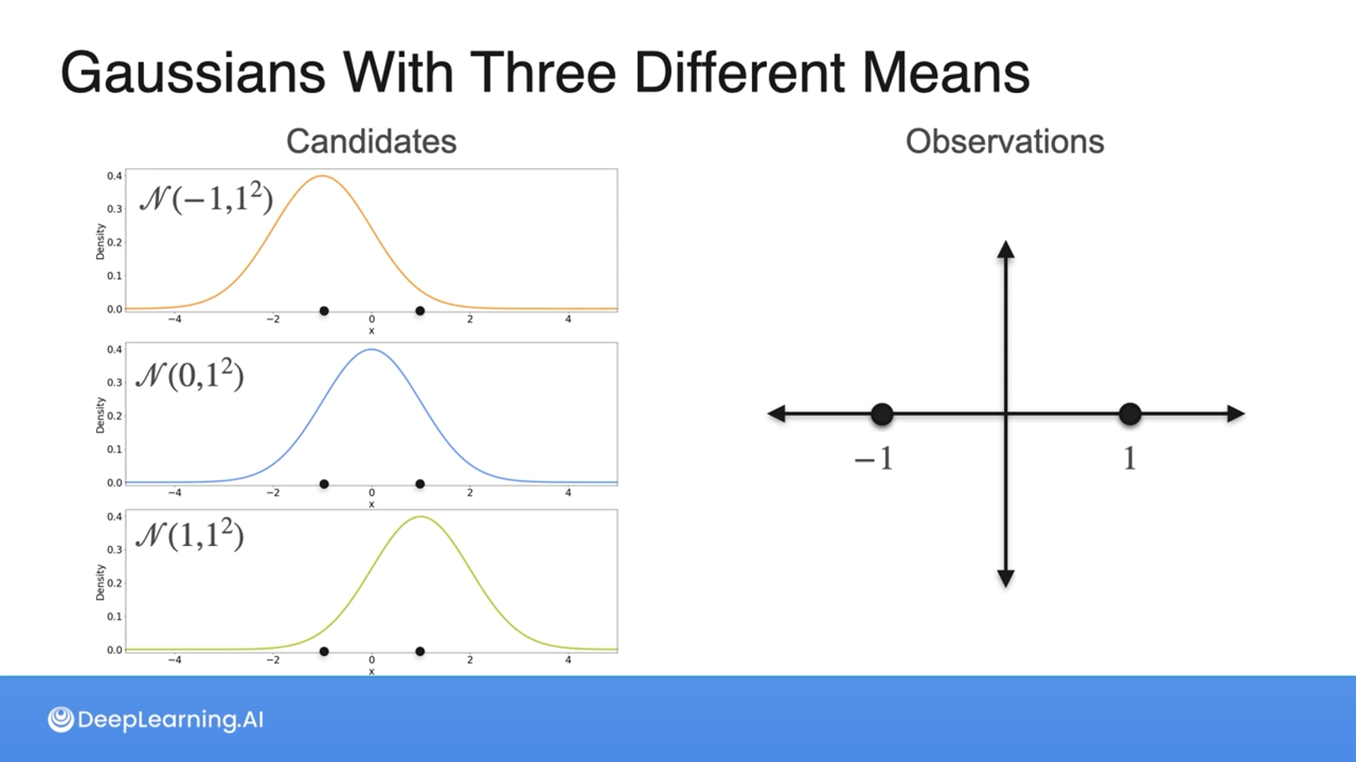
Given the sample {-1, 1} from an unknown Normal distribution, which one is more likely to have generated the sample?
- $N(-1,1^2)$
- $N(0,1^2)$
- $N(1,1^2)$
2
Correct! Of the three possibilities given, the Gaussian with mean 0 and variance 1 maximizes the chances of seeing the sample {-1, 1}
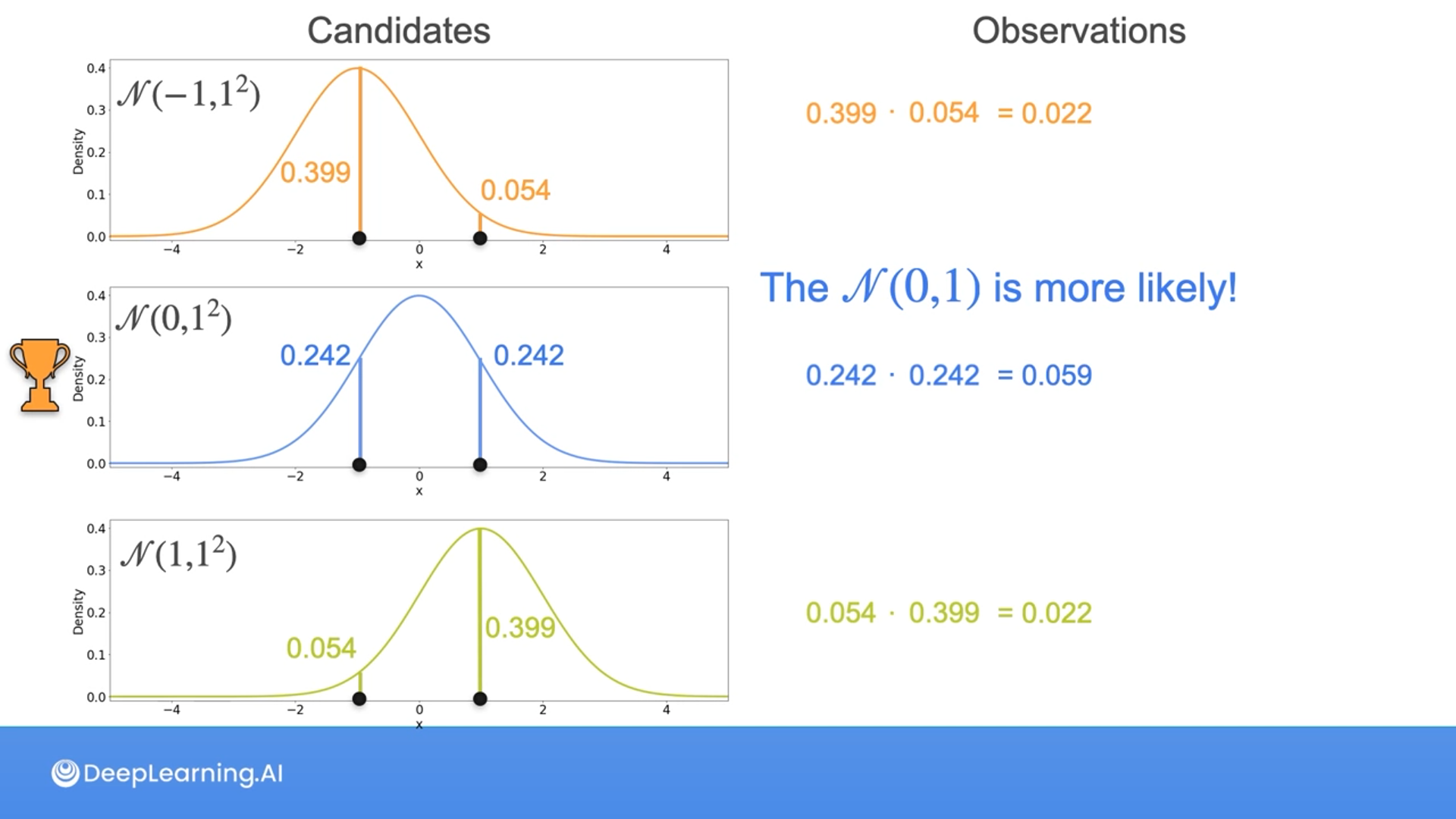
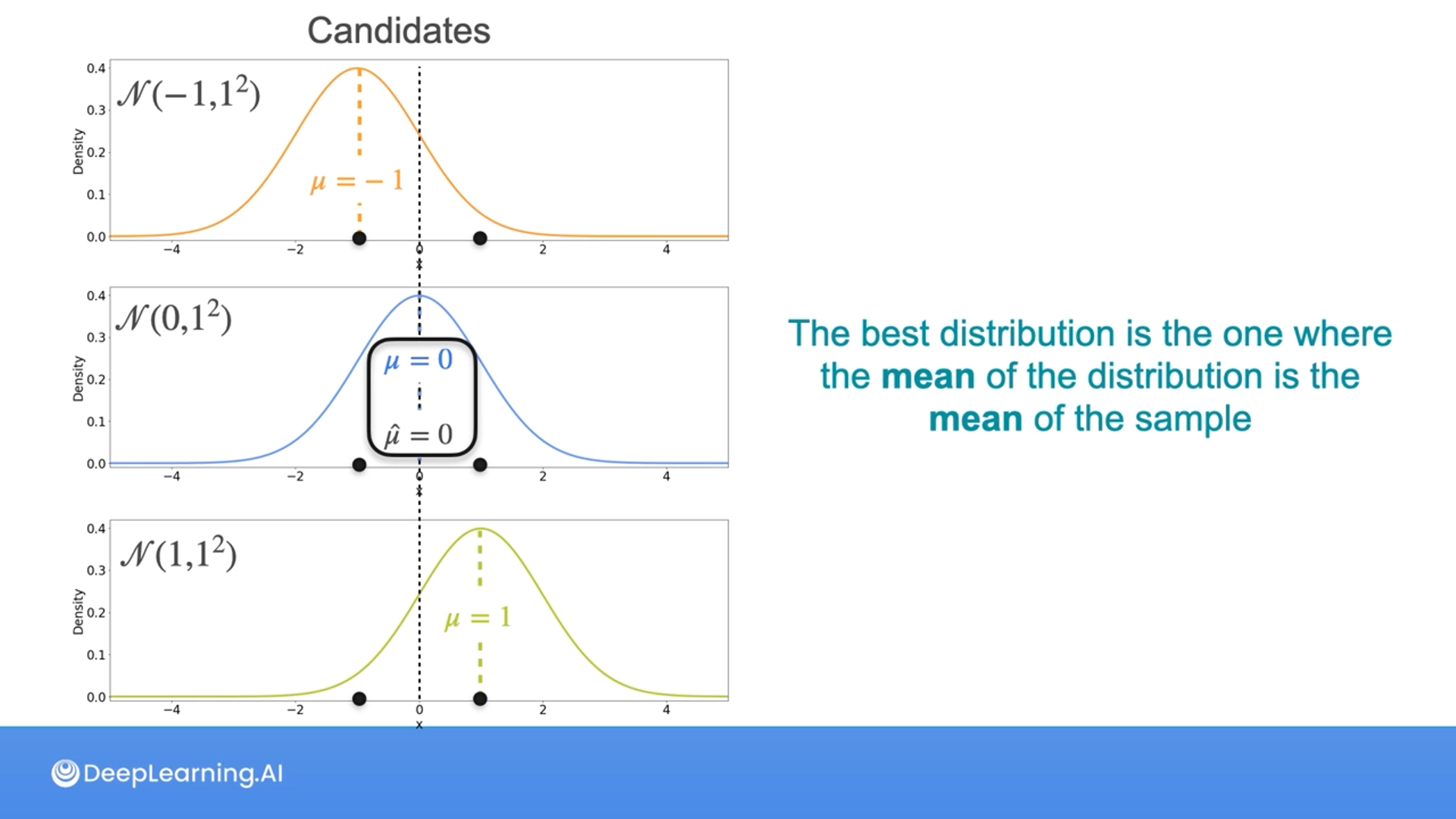
Notice that the mean of the original dataset is the same as the mean of the distribution with the maximum likelihood.

Given the sample {-1, 1} from an unknown Normal distribution, which one is more likely to have generated the sample?
- $N(0,0.5^2)$
- $N(0,1^2)$
- $N(0,2^2)$
2
Correct! Of the two possibilities given, the Gaussian with mean 0 and variance 1 maximizes the chances of seeing the sample {-1, 1}
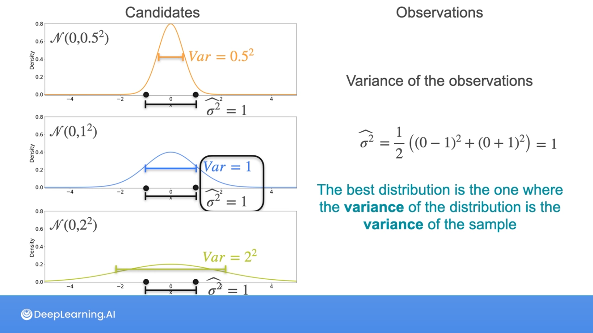
Here, Luis is dividing by 2 using the formula for population variance, not the sample variance as you saw in previous lectures. This is because, as mentioned, the population variance is biased, hence to obtain an unbiased estimator, it should be divided by n-1 instead of n. However, the maximum likelihood estimator (MLE) for the variance is biased and equals the population variance.
MLE for the Gaussian population
You have an intuition of what the Maximum Likelihood Estimation (MLE) should look like for the mean and variance of a Gaussian population.
Now you will learn the derivation of both results.
Mathematical formulation
Suppose you have $n$ samples $\boldsymbol{X}=\left(X_1, X_2, \ldots, X_n\right)$ from a Gaussian distribution with mean $μ$ and variance $σ^2$. This means that $X_i \stackrel{i . i . d .}{\sim} \mathcal{N}\left(\mu, \sigma^2\right)$.
If you want the MLE for $\mu$ and $\sigma$ the first step is to define the likelihood. If both $\mu$ and $\sigma$ are unknown, then the likelihood will be a function of these two parameters. For a realization of $X$, given by $x=(x_1, x_2, \dots, x_n):$
$$ \begin{aligned}L(\mu, \sigma ; \boldsymbol{x}) & =\prod_{i=1}^n f_{X_i}\left(x_i\right)=\prod_{i=1}^n \frac{1}{\sqrt{2 \pi} \sigma} e^{-\frac{1}{2} \frac{\left(x_i-\mu\right)^2}{\sigma^2}} \\& =\frac{1}{(\sqrt{2 \pi})^n \sigma^n} e^{-\frac{1}{2} \frac{\sum_{i=1}^n\left(x_i-\mu\right)^2}{\sigma^2}}\end{aligned} $$
Now all you have to do is find the values of $\mu$ and $\sigma$ that maximize the likelihood $L(\mu, \sigma; \boldsymbol{x})$.
You might remember from the calculus course that one way to do this analytically is by taking the derivative of the Likelihood function and equating it to 0. The values of $μ$ and $σ$ that make the derivative zero, are the extreme points. In particular, for this case, they will be maximums.
Taking the derivative of the likelihood is a cumbersome procedure, because of all the products involved. However, there is a nice trick you can use to simplify things. Note that the logarithm function is always increasing, so the values that maximize $L(μ,σ;\boldsymbol{x})$ will also maximize its logarithm. This is the log-likelihood, and it is defined as $\ell(\mu, \sigma)=\log (L(\mu, \sigma ; \boldsymbol{x}))$
The logarithm has the property of turning a product into a sum, this means that $\log(a\cdot b) = \log(a)+\log(b)$. This makes taking the derivative of the log-likelihood very straightforward. To get the simplest expression for the log-likelihood for a Gaussian population, you will also need the following properties of the logarithm:
$\log(1/a) = -\log(a)$
and
$\log(a^k)=k\log(a)$.
Putting it all together you get:
$$ \begin{aligned}\ell(\mu, \sigma)&=\log\left(\frac{1}{(\sqrt{2 \pi})^n \sigma^n} e^{-\frac{1}{2} \frac{\sum_{i=1}^n\left(x_i-\mu\right)^2}{\sigma^2}}\right)\\ &=-{n\over2}\log(2\pi)-n\log(\sigma)-{1\over2}{\sum_{i=1}^n(x_i-\mu)^2\over\sigma^2} \end{aligned} $$
Now to find the MLE for $\mu$ and $\sigma$, all there is left to do is to take the partial derivatives of the log-likelihood and equate them to zero.
For the partial derivative with respect to $μ$ note that the first two terms do not involve $μ$, so you get:
$$ \begin{aligned} {\partial\over\partial\mu}\ell(\mu, \sigma)&=-{1\over2}{\sum_{i=1}^n2(x_i-\mu)\over\sigma^2}(-1)\\ &={1\over\sigma^2}(\sum_{i=1}^nx_i-\sum_{i=1}^n\mu) = {1\over\sigma^2}(\sum_{i=1}^nx_i-n\mu) \end{aligned} $$
Now, for the partial derivative with respect to $\sigma$, you get that
$$ \begin{aligned} {\partial\over\partial\sigma}\ell(\mu, \sigma)=-{n\over\sigma}-{1\over2}\left(\sum_{i=1}^n(x_i-\mu)^2\right)(-2){1\over\sigma^3} = -{n\over\sigma}+\left(\sum_{i=1}^n(x_i-\mu)^2\right){1\over\sigma^3} \end{aligned} $$
The next step is equating this to 0 to find the estimates for $μ$ and $σ$. Let's begin with the partial derivative with respect to $μ$:
$$ {\partial\over\partial\mu}\ell(\mu, \sigma) = {1\over\sigma^2}(\sum_{i=1}^nx_i-n\mu) = 0 $$
First, observe that since $\sigma >0$, the only option is that $\sum_{i=1}^nx_i-n\mu = 0$. Simple algebraic manipulations show that the MLE for $\mu$ has to be
$$ \hat\mu={\sum_{i=1}^nx_i\over n} = \bar x $$
which is the sample mean.
Next, find the value of $\sigma$ that achieves ${\partial\over\partial\sigma}\ell(\mu, \sigma) = 0$:
$$ {\partial\over\partial\sigma}\ell(\mu, \sigma) =-{n\over\sigma}+\left(\sum_{i=1}^n(x_i-\mu)^2\right){1\over\sigma^3} =0 $$
In this case, first note that since $\sigma >0$, you can simplify the expression to
$$ {\partial\over\partial\sigma}\ell(\mu, \sigma) =-n+\left(\sum_{i=1}^n(x_i-\mu)^2\right){1\over\sigma^2} =0 $$
Also, you can replace $\mu$ with its estimate $\hat\mu=\bar x$, because you want both partial derivatives to be 0 at the same time. So you get
$$ {\partial\over\partial\sigma}\ell(\mu, \sigma) =-n+\left(\sum_{i=1}^n(x_i-\bar x)^2\right){1\over\sigma^2} =0 $$
This gives you
$$ \sigma^2={\sum(x_i-\bar x)^2\over n} $$
so the MLE for the standard deviation is
$$ \hat\sigma=\sqrt{\sum(x_i-\bar x)^2\over n} $$
This expression tells you that the MLE for the standard deviation of a Gaussian population is the square root of the average squared difference between each sample and the sample mean. This expression is very similar to the one you learned in Week 2 for the sample standard deviation. The only difference is the normalizing constant: for the MLE you have $1/n$ while for the sample standard deviation, you use $1/(n-1)$.
A final comment: formally, what you just did was the derivation of the critical point. To make it all complete, you would need to show that these are the coordinates of a maximum point (and not a minimum or saddle point). However, this proof would require a little bit more complicated math and we will skip it here.
A simple example
Now, let's see what this looks like with an example. Suppose you are interested in the distribution of heights of 18-year-olds in the US. You have the following 10 measurements:
$$ 66.75\quad70.24\quad67.19\quad67.09\quad63.65\\ 64.64\quad69.81\quad69.79\quad73.52\quad71.74 $$
Each measurement is supposed to come from a Gaussian distribution with unknown parameters $μ$ and $σ$. The MLE estimation for the parameters with these samples are
$$ \begin{aligned} \hat\mu&={66.75+70.24+67.19+67.09+63.65+64.64+69.81+69.79+73.52+71.74\over10}\\&=68.442 \end{aligned} $$
and
$$ \begin{aligned} \hat\sigma&=\sqrt{{1\over10}\left((66.75-68.442)^2+(70.24-68.442)^2+(67.19-68.442)^2+\\ (67.09-68.442)^2+(63.65-68.442)^2+(64.64-68.442)^2+\\ (69.81-68.442)^2+(69.79-68.442)^2+(73.52-68.442)^2+(71.74-68.442)^2\right)}\\ &=2.954 \end{aligned} $$
TL; DR;
After all the calculations using derivatives to find the MLE for $\mu$ and $\sigma$, $\hat\mu$ is the sample mean and $\hat\sigma$ is the sample variance without the $-1$ part in the denominator
MLE: Linear Regression

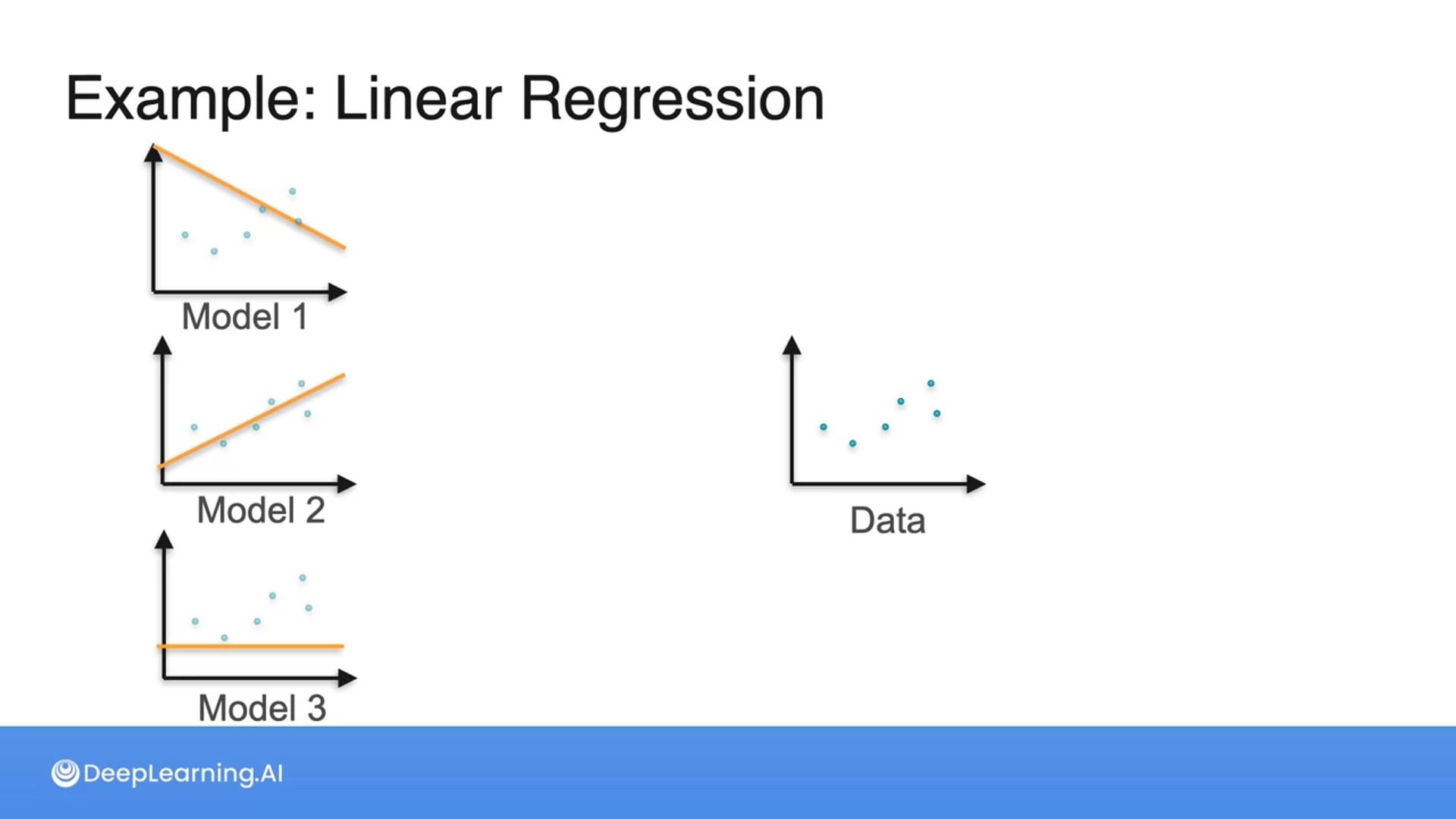
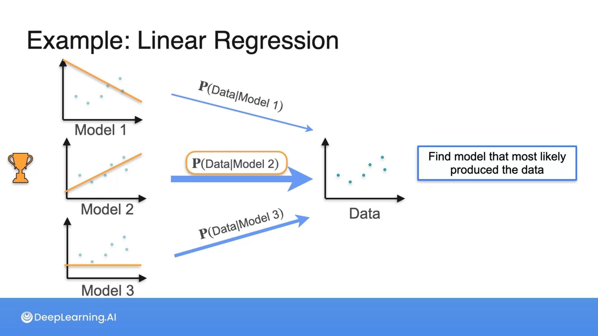
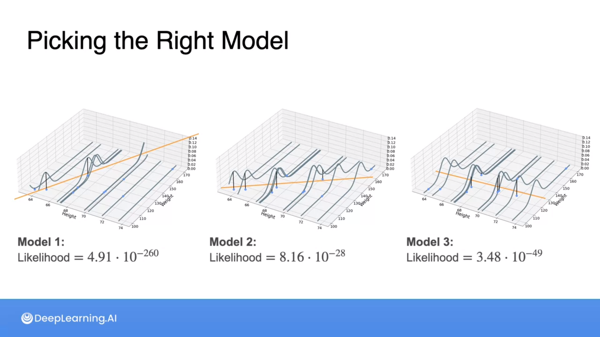
Which of the following models best fits the data?
Model 2
Great job! When choosing the most appropriate model for a dataset, assess how well each model visually clusters or captures the distribution of data points to ensure it accurately represents the observed data pattern.
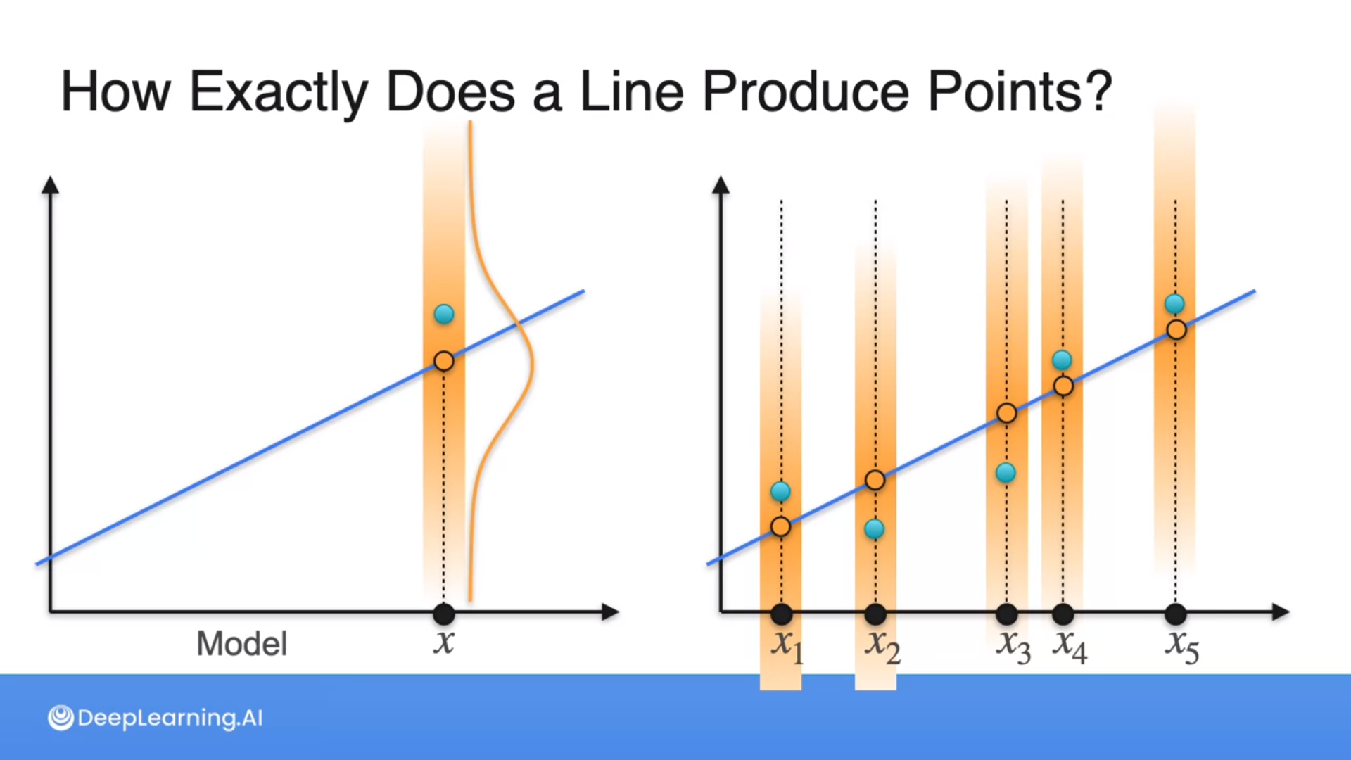
At points, we generate random points using the Gaussian distributions.
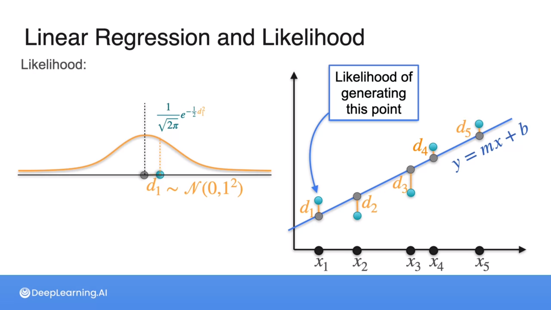
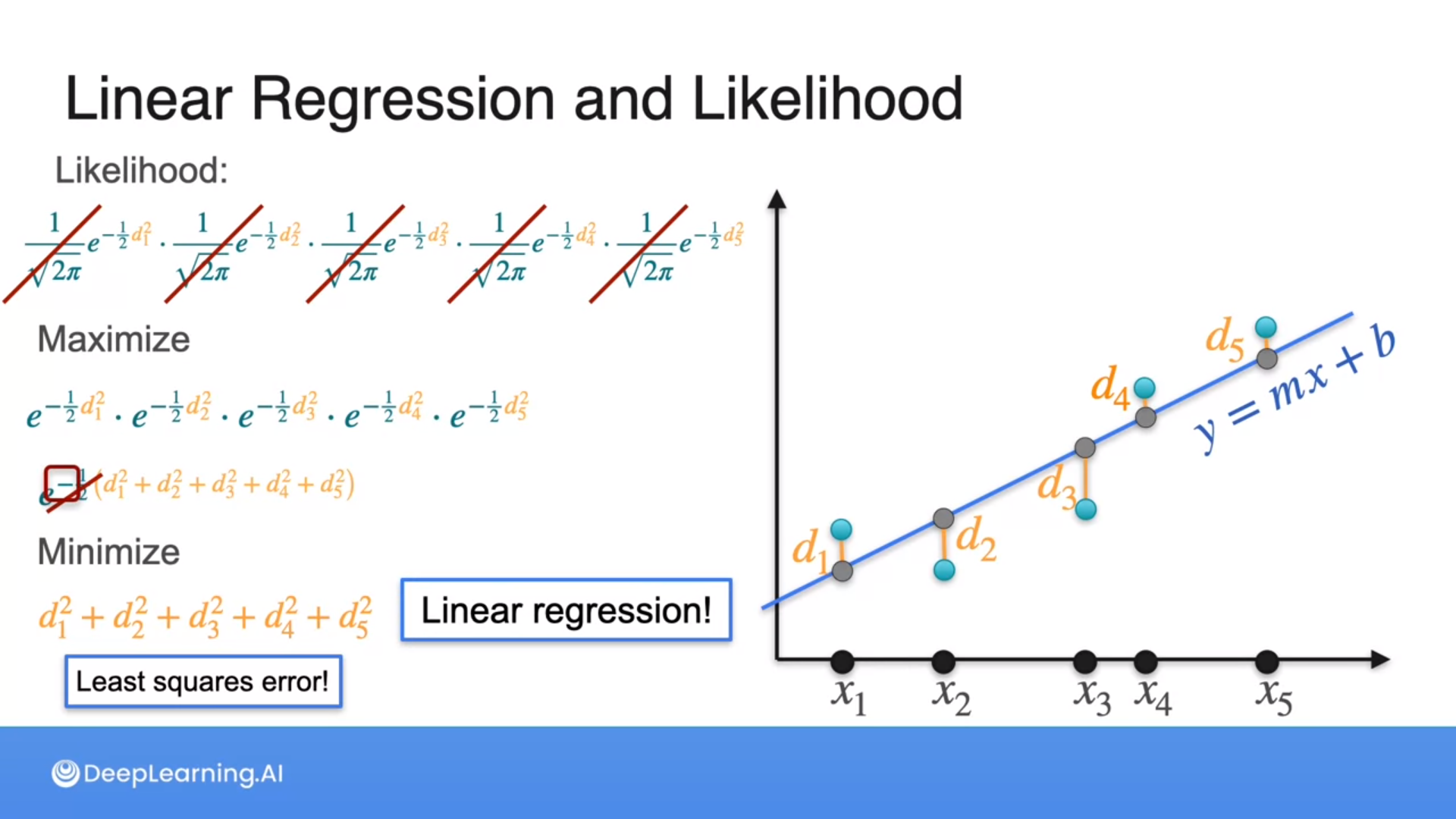
Maximizing the likelihood of distances of points from a line is the same as minimizing the least squares error, which is the goal of linear regression.
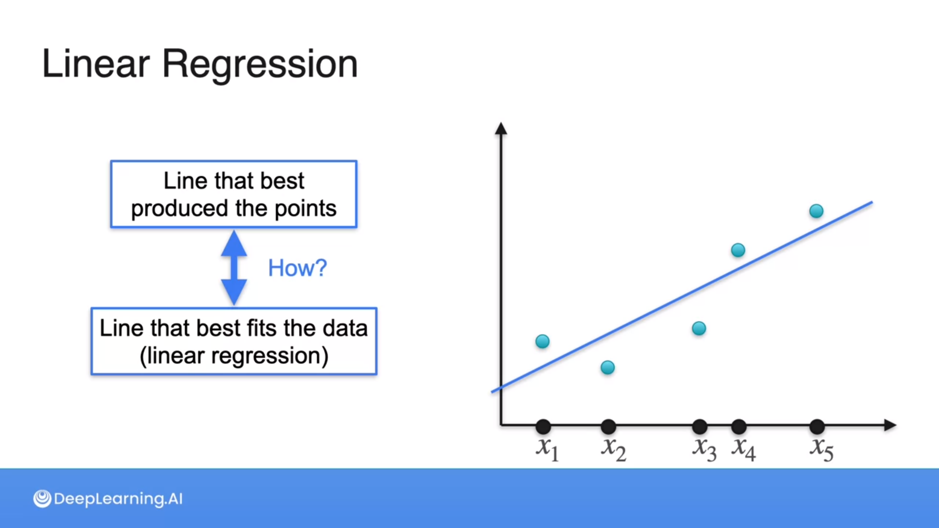
Hence, picking the line that best produces the points is the same as the line that best fits the data (linear regression).
Regularization
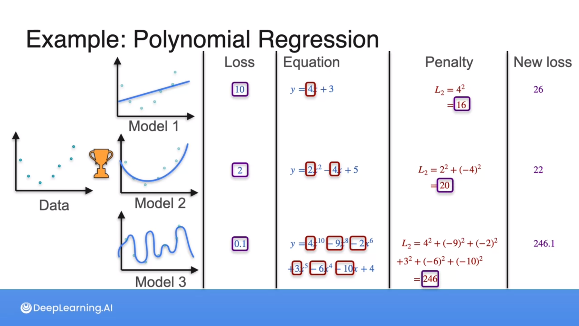
The more complicated, the higher the penalty we apply to the model.
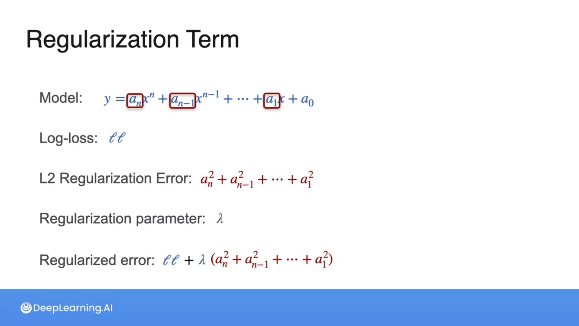
L2 regularization (penalty) will be the sum of the squares of all the coefficients of the polynomial.
How do you account for penalty and loss values when determining the best model with regularization?
- Calculate the new loss as the sum of the penalty and the previous loss.
- Set the new loss equal to the penalty value.
1
That's right! When incorporating regularization into the loss function, the penalty term is added to the previous loss to form the new loss. This ensures that the penalty for complexity is appropriately balanced with the original loss.
Why is regularization important in machine learning?
- To increase the complexity of the model.
- To prevent overfitting and improve generalization.
- To introduce randomness into the model.
2
Regularization techniques help prevent overfitting by adding a penalty term to the loss function, which discourages overly complex models. This improves the model's ability to generalize well to unseen data.
All the information provided is based on the Probability & Statistics for Machine Learning & Data Science | Coursera from DeepLearning.AI


