▤ 목차
Describing probability distributions and probability distributions with multiple variables
Probability Distributions with Multiple Variables
Covariance of a Dataset
To capture the relation between variables using covariance and correlation.

How might you compare the relationship between a child's age (X) and other variables such as height (Y1), test grades (Y2), and number of naps per day(Y3)?
Create a scatter plot to examine the relationship between age and each variable visually.


Computing the mean or the variance doesn’t help find the relationship between variables.


One way is by computing the covariance.


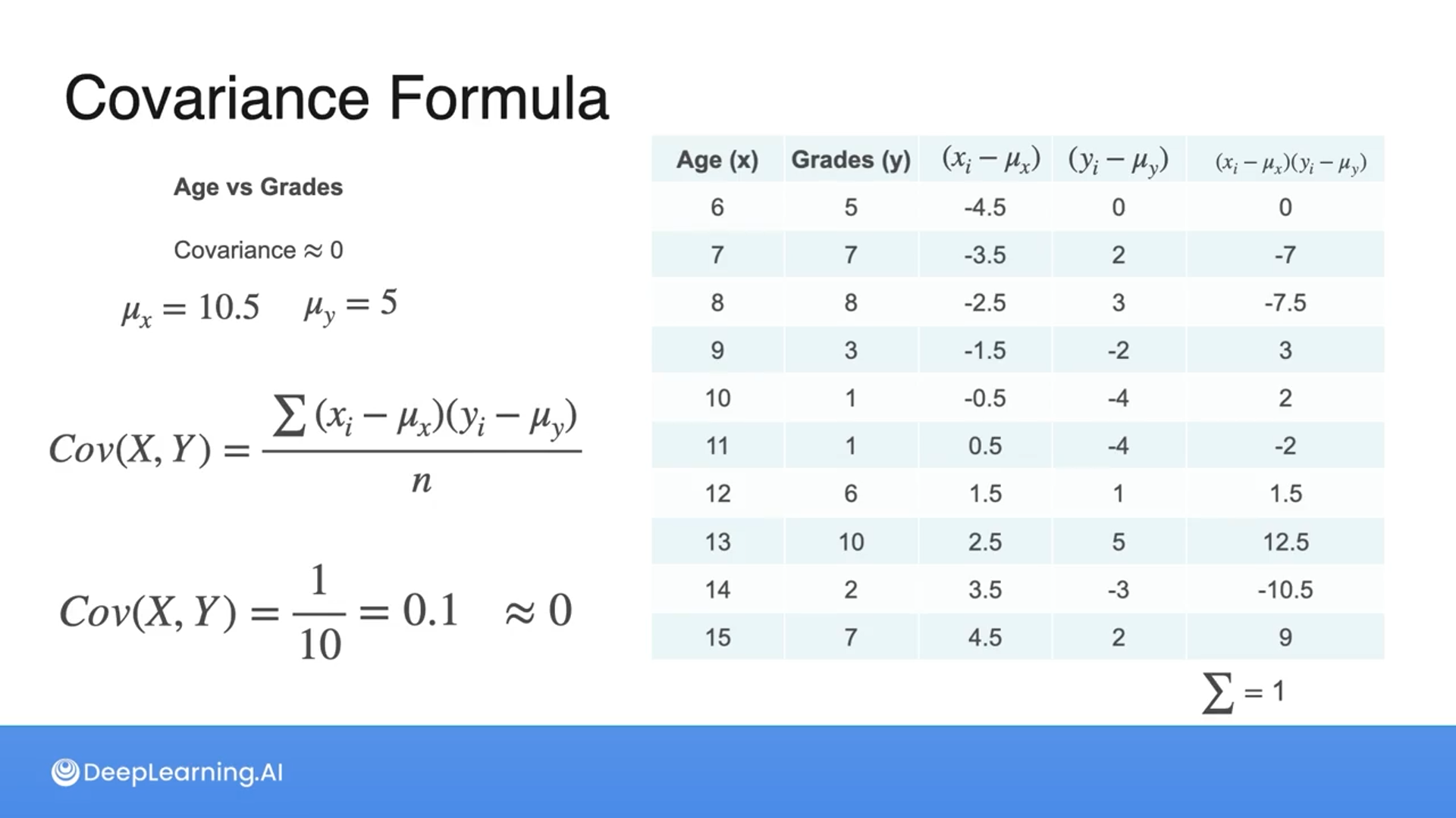
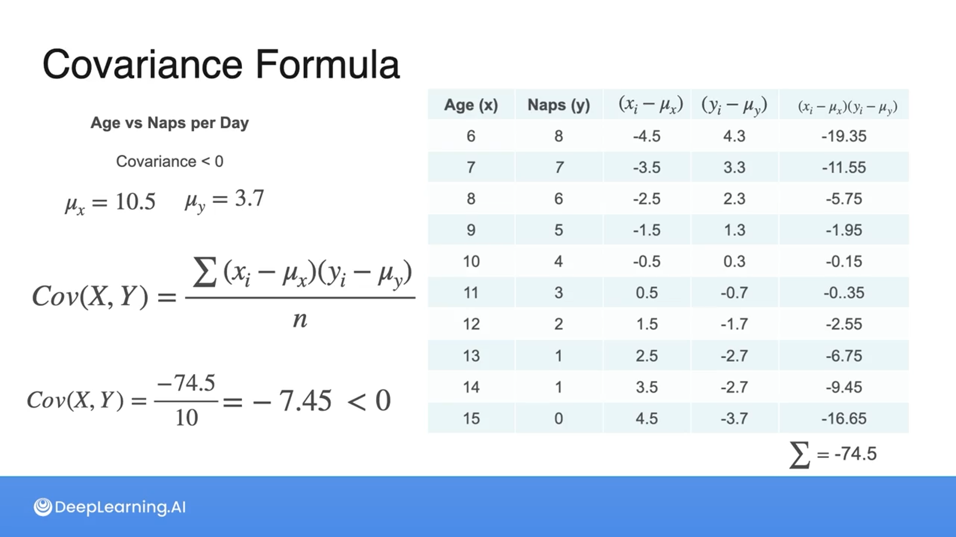

You compare a dataset X and Y and obtain a covariance value of 10. What does this value tell you?
There is a positive relationship between X and Y.
A covariance value of 10 indicates a positive relationship between X and Y. The magnitude of the covariance suggests that the relationship is relatively strong.
Covariance of a Probability Distribution
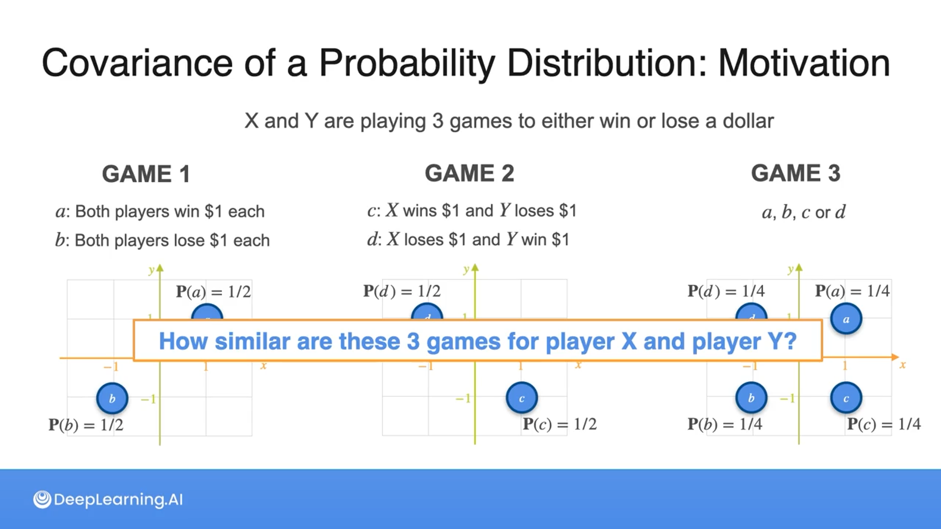


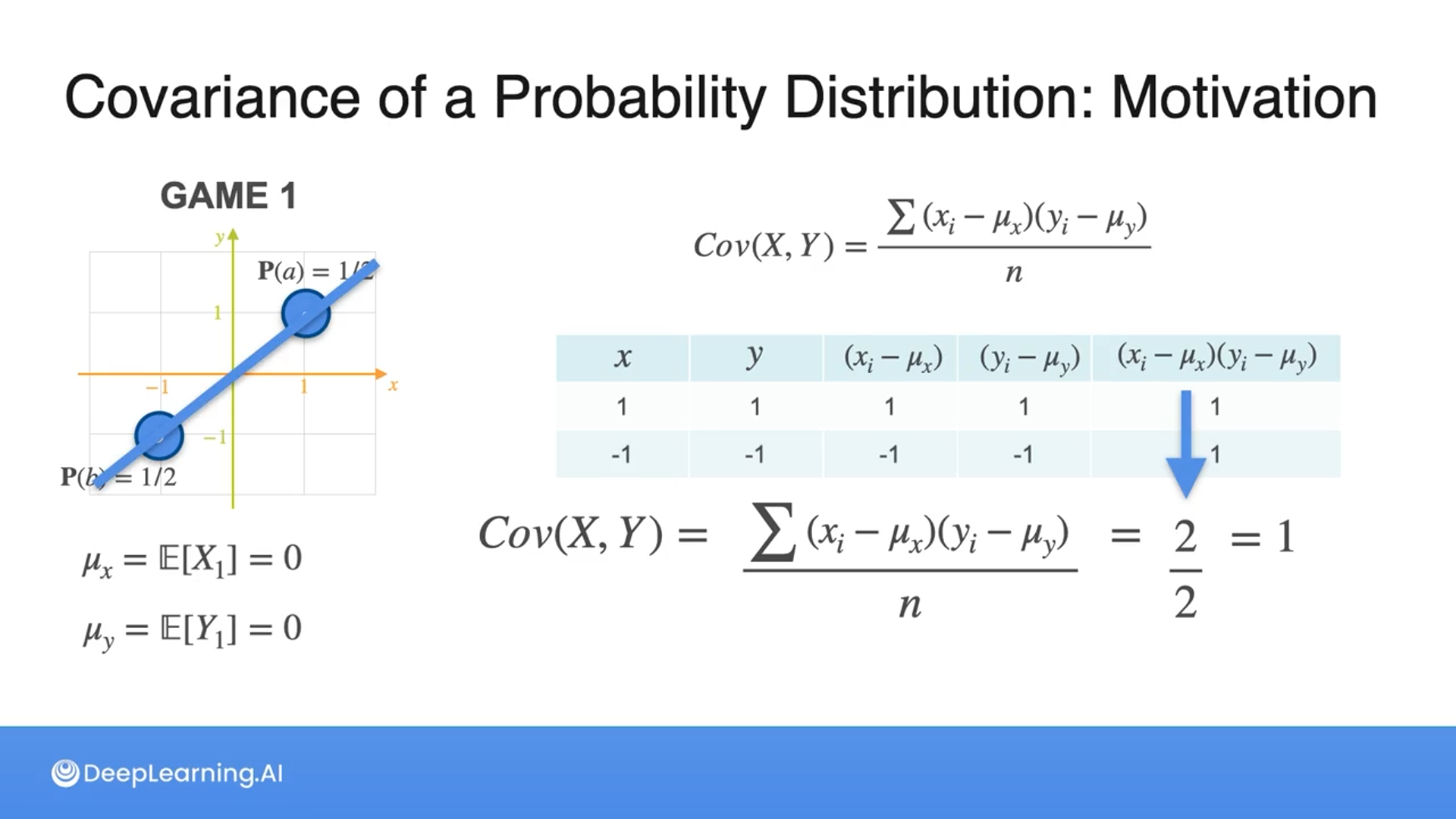
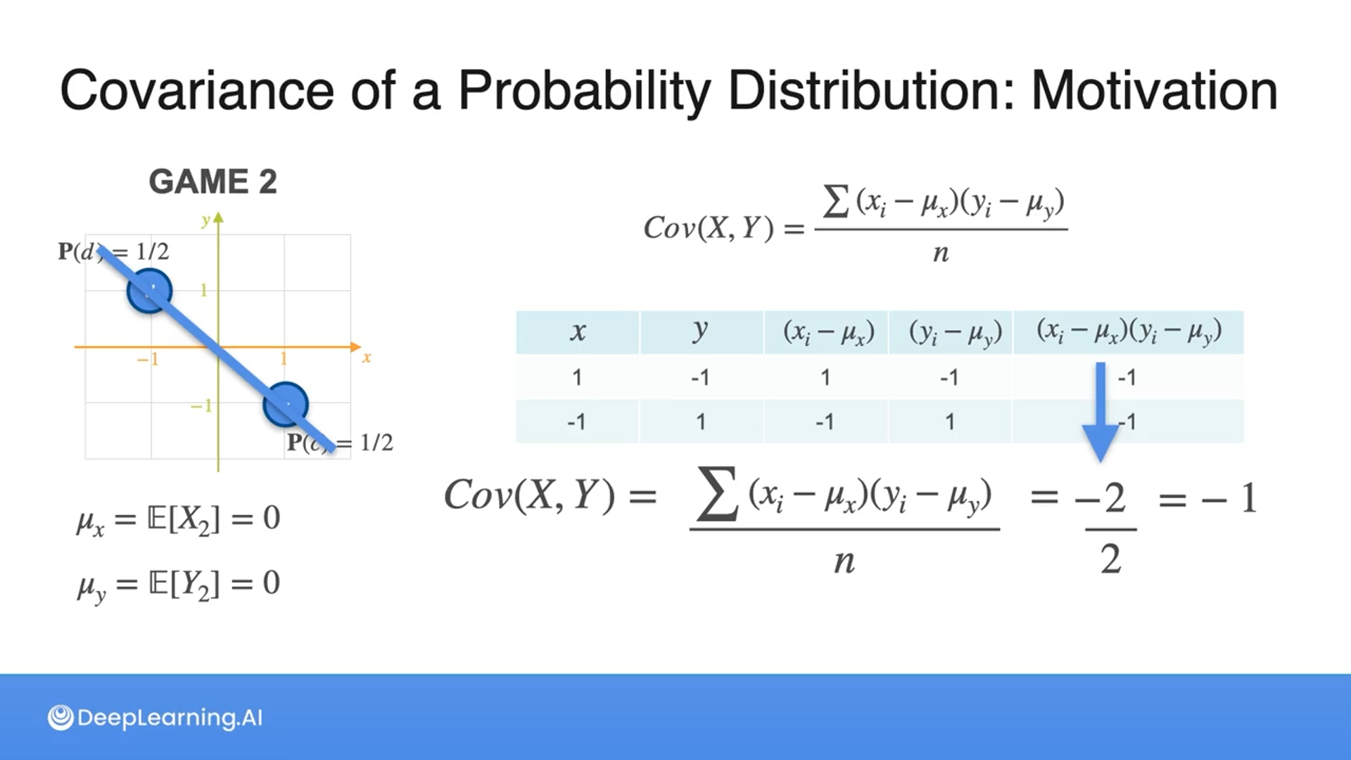


Here we can see how covariance can be used to compare variables when neither mean nor variance shows the relationship when they have equal probabilities.
What happens to the covariance if the probabilities are not equal?

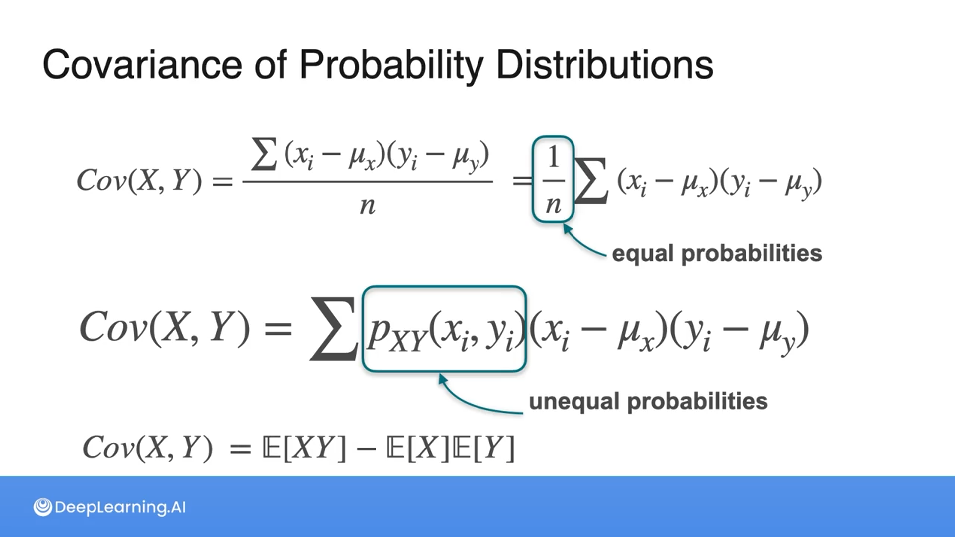


Then we multiply by each probability after subtracting the mean (refer to the second and third slides) instead of dividing by n (the number of samples).
Covariance Matrix
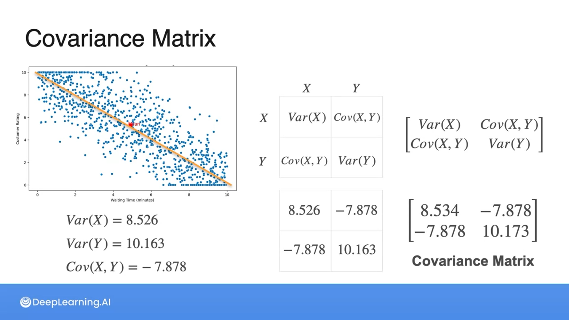


A covariance matrix is a matrix with the variances and covariances of each variable in a matrix format.
Correlation Coefficient


We can tell the relationship between variables with covariance, but not which one is stronger.
With the correlation coefficient, we can tell which one has a stronger relationship, which is the standardized covariance.
To get the correlation coefficient we multiply the standard deviations (square root of the variance) of variables and divide the output from the covariance.
The correlation coefficient falls between -1 and 1 where:
- -1 means negative correlation
- 0 means uncorrelated
- 1 means the positive correlation
Multivariate Gaussian Distribution


If two variables are independent, then the joint PDF (probability density function) would be the product of the marginal PDFs.
When the variables are dependent the plot would be elongated due to having covariance (one variable having a relation to another variable).
The only change in the formulas between the independent and dependent cases is that the diagonal matrix in the independent case updates to have covariances between variables.


For multivariate Gaussian distributions, instead of dividing by the square root of 2 pi, we divide by 2 pi to the power of n/2, taking into account the number of variables.
And standard deviation updates to the determinant of the covariance matrix to the power of 1/2, which captures the volume of the spread, as it tells us the variation in the curve.
The bigger the determinant, the bigger the spread.
All the information provided is based on the Probability & Statistics for Machine Learning & Data Science | Coursera from DeepLearning.AI


 }
}