▤ 목차
Describing probability distributions and probability distributions with multiple variables
Probability Distributions with Multiple Variables
Joint Distribution (Discrete) - Part 1
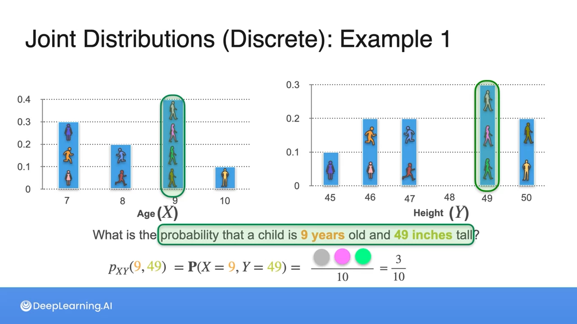
Here we have two histograms of children’s age and height (two variables).


Given the following dataset, what is the probability that a child is 9 years old and 49 inches tall?
0.3

Getting the count and probabilities in a table format like the one below is easier.


Joint Distribution (Discrete) - Part 2


When the discrete random variables are independent, we multiply the probabilities.


If they are not independent, we can use a histogram to get the count and probabilities.
We divide the count by the total number of possible outcomes for dependent joint distributions.
Joint Distribution (Continuous)


Remember that we have to put the data in ranges or intervals as continuous values can have an infinite number of values that cannot be measured when treated individually.
We can visualize joint distributions of continuous variables in the form of histograms, heat maps, scatter plots, and density plots.


What is the difference between preparing a joint distribution for discrete versus continuous variables?
- Discrete joint distributions assign probabilities to individual outcomes, while continuous joint distributions assign probabilities to ranges or intervals of values.
- Discrete joint distributions have a countable or finite number of possible outcomes, while continuous joint distributions have an uncountably infinite number of possible outcomes.
- Discrete joint distributions are typically represented by scatter plots, while continuous joint distributions are represented by bar charts.
Answer
1, 2
Marginal and Conditional Distribution
Marginal distribution is when we aggregate all the data on certain feature(s).
- It’s like reducing a dimension or fixing (focusing on) one variable.
Conditional distribution is when we slice the data to a certain value of a certain feature(s).
- It’s like filtering the data.

Create a table to represent the marginal distribution for Height(Y).
| Height (Y) | 45 | 46 | 47 | 48 | 49 | 50 |
| Probability | 1/10 | 2/10 | 2/10 | 0 | 3/10 | 2/10 |


What is the formula for $p_Y(50)$?
$p_Y(50)=\sum_ip_{XY}(x_i, 50)={2\over10}$


The way we get the marginal distribution for the continuous variables is the same, we aggregate the data along the axis we want to focus on.
Conditional Distribution
Conditional Distribution is used when we want to find the distribution across one variable when the other one is given.
To do that we have to normalize the data by the marginal distribution of the given variable.


What is the value of P(Y=46 | X=7)?
2/3

The above formula is like a specific probability (the probability we want) divided by the sum of row or column probabilities.
We are applying the conditional probability rule when we normalize.


The formula for the continuous conditional distribution stays the same, except we use the PDF (Probability Density Function) instead of PMF (Probability Mass Function).
All the information provided is based on the Probability & Statistics for Machine Learning & Data Science | Coursera from DeepLearning.AI


